Random Matrix Theory
Here, we discuss some selected topics and techniqes from random matrix theory. For sake of clarity, we will first deal with 1-matrix models, and illustrate how they count the number of planar diagrams in a certain limit. Then, we discuss the 2-matrix models, which enumerate 2-colored planar diagrams. For this, we will need the Harish-Chandra (Itzykson-Zuber) formula, which we also derive. Before discussing the connections of these matrix models to enumeration problems, we first derive some basic facts about the space of Hermitian matrices that we will eventually need in order to perform calculations.
We will always let $\mathcal{H}$n denote the space of $n\times n$ Hermitian matrices, i.e. matrices $X$ such that $X^\dagger = X$ ("$\dagger$" here denotes hermitian conjugate). The dimension of this space may be computed by noticing the following: the hermiticity condition requires that the diagonal of the matrix be real ($z = \bar{z}$ implies that $z$ is real), therefore the diagonal entries contribute $n$ variables. Above the diagonal, there are $2 \cdot \frac{n(n-1)}{2} = n (n-1)$ variables (the factor of two coming from real + imaginary components); therefore we find the dimension of the space of Hermitian matrices to be \begin{align} \dim H_n = n + 2 \cdot \frac{n(n-1)}{2} = n^2. \end{align} It is often convenient for us to work in the so-called eigenvalue variables on the space of Hermitian matrices. These eigenvalues are of course real, by properties of Hermitian matrices; the remaining variables are variables in the unitary group $U(n)/U_{diag}(n)$ and are called angular variables. This is apparent, by writing $X = U^\dagger \Lambda U$; note that replacing $U \to \text{diag}(e^{i\theta_1},\cdots e^{i\theta_n} )U$ does not change the representation. Defining $du := dU^\dagger U = -du^{\dagger}$, we find that $dX$ takes the form \begin{align*} dX = d(U^\dagger \Lambda U) &= dU^\dagger \Lambda U+ U^\dagger d\Lambda U + U^\dagger \Lambda dU \\\ &= U^\dagger (d u^\dagger \Lambda + d \Lambda + \Lambda d u) U \\\ &= U^\dagger (d \Lambda + [\Lambda, d u] ) U. \end{align*}
The metric can then be computed as \begin{align*} g = \text{tr} (dX^\dagger dX) = \text{tr}(d \Lambda d \Lambda) + \text{tr}([\Lambda, d u])^2, \end{align*} which is diagonal in the coordinates $(d\lambda_i, du_{ij})$: \begin{align*} g = \sum_{i = 1}^n d\lambda_i^2 + 2 \sum_{i < j} (\lambda_i - \lambda_j)^2 (du_{ij})^2 \end{align*} The volume form is then \begin{align*} d\text{vol}(X) &= \sqrt{\det g} \prod_{i=1}^n d\lambda_i \prod_{i < j} du_{ij} \\\ &= 2^{n(n-1)} \prod(\lambda_i - \lambda_j)^2 \prod_{i=1}^n d\lambda_i \prod_{i < j} du_{ij} \\\ &\propto dU \prod_{i < j}(\lambda_i - \lambda_j)^2 \prod_{i=1}^n d\lambda_i, \end{align*} where $dU$ is the Haar measure on $U(n)/U_{diag}(n)$. The quantity \begin{equation} V(\lambda) := \prod_{i < j}(\lambda_i - \lambda_j) = \det(\lambda_i^{j-1}) \end{equation} is called the Vandermonde determinant. We shall meet it often later. The exponent of two in the Vandermonde determinant comes from the fact that there are twice as many variables $du_{ij}$, with contributions coming from real and imaginary parts, respectively. Because it is a quantity we will need later, we also compute the Laplace-Beltrami operator on the submanifold of the eigenvalue coordinates; this is \begin{align*} \Delta_{LB} &= \sum_{i=1}^n \frac{\partial^2}{\partial X_{ii}^2} + \frac{1}{2}\sum_{i < j}\left(\frac{\partial^2}{\partial \text{Re}(X_{ij})^2} + \frac{\partial^2}{\partial \text{Im}(X_{ij})^2}\right)\\\ &= \frac{1}{V^2(\lambda)}\sum_{i=1}^n\frac{\partial}{\partial \lambda_i} \left(V^2(\lambda) \frac{\partial}{\partial \lambda_i} \cdot\right) + (\Delta \textit{ on the angular coordinates}), \end{align*} i.e., on only the eigenvalue coordinates, we have \begin{equation}\label{eigenvalue-laplacian} \Delta_{eigenvalues} = \frac{1}{V^2(\lambda)}\sum_{i=1}^n\frac{\partial}{\partial \lambda_i} \left(V^2(\lambda) \frac{\partial}{\partial \lambda_i} \cdot\right). \end{equation}
$1$. The Gaussian Unitary Ensemble & Planar Diagrams.
We now demonstrate how certain integrals over $\mathcal{H}$n can be related to enumeration of planar diagrams, a fact which was first noticed by the physicists E. Brezin, C. Itzykson, G. Parisi, & J. B. Zuber. Most of the results presented here are standard; they can be found in places like this paper by Phillipe Di Francesco, or in this one by Alexander Zvonkin, for example. Let $\mathcal{H}$n denote the space of $n\times n$ Hermitian matrices. We consider the measure \begin{equation*} d\mathbb{P}(X) = \frac{1}{Z_n} e^{-\frac{n}{2}\text{tr} X^2} dX, \end{equation*} where $dX$ is Haar measure on $\mathcal{H}$n (which we have just defined in the previous section), and $Z_n$ is a normalization constant so that $\int d\mathbb{P} = 1$, called the \textit{partition function}. The ensemble of such matrices, taken together with the probability measure $\mathbb{P}$n, form the Gaussian Unitary Ensemble (GUE). We denote the expected value of a random variable $f(X):$ $\mathcal{H}$n $\to \mathbb{R}$ in this ensemble by $\langle f(X) \rangle_n$; explicitly, \begin{equation} \langle f(X) \rangle_n = \frac{1}{Z_n} dX \int_{H_n} f(X) e^{-\frac{n}{2}\text{tr} X^2}. \end{equation} We wish to evaluate expected values of certain random variables in the large $n$ limit, in particular (Notice that $X\in \mathcal{H}$n is dependent on $n$ as well; we suppress dependence to simplify notations.) \begin{equation} \langle \text{tr} X^k \rangle:= \lim_{n\to \infty} \frac{1}{n}\langle \text{tr} X^k \rangle_n. \end{equation} We claim that \begin{equation} \langle \text{tr} X^k \rangle = C_k, \end{equation} where $C_k = \frac{1}{k+1}{2k \choose k}$ is the $k^{th}$ Catalan number. This will follow from some combinatorial arguments. We begin by proving the following:
Theorem 1.1 Let $S\in \mathcal{H}_n$ be a fixed matrix. Then, \begin{equation} \langle e^{\text{tr} XS}\rangle_n = e^{\text{tr} S^2/2n}. \end{equation}
Proof. We have that \begin{align*} \langle e^{\text{tr} XS} \rangle_n &= \frac{1}{Z_n}\int_{H_n}dX e^{-\frac{n}{2}\text{tr} (X^2 - \frac{2}{n} XS)}\\\ &= e^{\text{tr} S^2/2n} \frac{1}{Z_n}\int_{H_n}dX e^{-\frac{n}{2}\text{tr} (X-S/n)^2} \\\ &=e^{\text{tr} S^2/2n} \frac{1}{Z_n}\int_{H_n}d(X-S/n) e^{-\frac{n}{2}\text{tr} (X-S/n)^2}\\\ &= e^{\text{tr} S^2/2n} \frac{1}{Z_n}\int_{H_n}dX e^{-\frac{n}{2}\text{tr} (X)^2} = e^{\text{tr} S^2/2n}, \end{align*} where in the last step, we used the fact that $dX$ is translation invariant.
Consequentially, we can compute any expected value of interest by differentiating $f(S) := e^{\text{tr} S^2/2n}$ with respect to $S$, and evaluating at $S=0$. For example, \begin{align} \langle X_{ij} \rangle_n = \frac{\partial f(S)}{\partial S_{ji}} \bigg|_{S=0}, \end{align}
and \begin{align} \langle X_{i_1j_1}X_{i_2j_2} \rangle_n = \frac{\partial^2 f(S)}{\partial S_{j_1i_1}\partial S_{j_2i_2}} \bigg|_{S=0}. \end{align}
Explicitly, we have that
Lemma 1.1 For any indices $i_1,j_1,i_2,j_2$, \begin{equation} \langle X_{i_1j_1} \rangle_n = 0, \qquad \qquad \langle X_{i_1j_1}X_{i_2j_2}\rangle_n = \frac{1}{n} \delta_{i_1 j_2}\delta_{i_2 j_1}. \end{equation} Proof. Note that the exponent of $f(S)$ is $\frac{1}{2n}\text{tr} S^2 = \frac{1}{2n}\sum_{k,l} S_{kl}S_{lk}$, and that \begin{equation*} \frac{\partial}{\partial S_{j_1 i_1}}\frac{1}{2n}\sum_{k,l} S_{kl}S_{lk} = \frac{1}{2n}\sum_{k,l} \left(\delta_{k j_1}\delta_{l i_1} S_{lk} + S_{kl}\delta_{l j_1}\delta_{k i_1}\right) = \frac{1}{n}S_{i_1 j_1}. \end{equation*} Therefore, by the chain rule, \begin{align} \langle X_{i_1j_1}\rangle_n = \frac{\partial}{\partial S_{j_1 i_1}}e^{\text{tr} S^2/2n}=\frac{1}{n}S_{i_1 j_1}e^{\text{tr} S^2/2n}\bigg|_{S=0} = 0. \end{align}
Similarly, by the product rule, \begin{align*} \langle X_{i_1j_1}X_{i_2j_2} \rangle_n &= \frac{\partial}{\partial S_{j_2 i_2}}\frac{1}{n}S_{i_1 j_1}e^{\text{tr} S^2/2n}\bigg|{S=0} \\\ &= \frac{1}{n}\delta{i_1 j_2}\delta_{i_2 j_1}e^{\text{tr} S^2/2n}\bigg|{S=0} + \frac{1}{n}S{i_1 j_1}S_{i_2 j_2}e^{\text{tr} S^2/2n}\bigg|{S=0}\\\ &= \frac{1}{n}\delta{i_1 j_2}\delta_{i_2 j_1}. \end{align*}
Furthermore, any “higher” expected value can be computed via Wick’s theorem}:
Theorem 1.2. (Wick’s Theorem.) Let $I = {(i_1,j_1),\cdots (i_{2M},j_{2M})}$ be a collection of indices, $1 \leq i_k,j_k \leq n$. Then, \begin{equation} \langle \prod_{(i,j) \in I}X_{ij} \rangle_n = \sum_{\pi \in \Pi_{2M}} \prod_{(i,j),(k,l)\in \pi} \langle X_{i j}X_{k l}\rangle_n, \end{equation} where $\Pi_{2M}$ is the set of all pairings of the index set $I$.
For example, we have that \begin{align*} \langle X_{i_1 j_1} X_{i_2 j_2} X_{i_3 j_3} X_{i_4 j_4}\rangle_n &= \langle X_{i_1 j_1} X_{i_2 j_2}\rangle_n \langle X_{i_3 j_3} X_{i_4 j_4}\rangle_n\\\ &+\langle X_{i_1 j_1} X_{i_3 j_3}\rangle_n \langle X_{i_2 j_2} X_{i_4 j_4}\rangle_n\\\ &+ \langle X_{i_1 j_1} X_{i_4 j_4}\rangle_n\langle X_{i_2 j_2} X_{i_3 j_3}\rangle_n. \end{align*}
Proof. (Sketch.) The theorem follows from the fact that derivatives must come in pairs for nonzero contributions to the expected value to appear; see the proof of the lemma. It is clear that the sum must be taken over all such pairings. The full proof of this fact is given in Zvonkin’s survey.
Corollary 1.1 The expected value of the product of an odd number of matrix elements is necessarily zero.
Using the above theorems, we are now able to compute expected values of quantities like $\langle \text{tr} X^k \rangle_n$. By the corollary, we trivially have that $\langle \text{tr} X^{2k+1}\rangle_n = 0$; it remains to compute the traces of even powers. This can be accomplished by realizing the pairings in Wick’s theorem as sums over families of $1$- face maps. We briefly summarize these results. Let us begin by way of example. Consider the expected value $\langle\text{tr} X^4 \rangle_n$; we have that, by linearity of $\langle \cdot \rangle_n$: \begin{equation*} \langle \text{tr} X^4 \rangle_n = \sum_{i_1, \cdots, i_4} \langle X_{i_1 i_2} X_{i_2 i_3} X_{i_3 i_4} X_{i_4 i_1} \rangle_n. \end{equation*} Using Wick’s theorem, we see that there are $3$ contributing terms in the above sum: \begin{align*} \langle X_{i_1 i_2} X_{i_2 i_3}\rangle_n &\langle X_{i_3 i_4} X_{i_4 i_1}\rangle_n,\quad \langle X_{i_1 i_2} X_{i_3 i_4}\rangle_n \langle X_{i_2 i_3} X_{i_4 i_1}\rangle_n,\quad \text{and }\\\ &\langle X_{i_1 i_2} X_{i_4 i_1}\rangle_n \langle X_{i_2 i_3} X_{i_3 i_4}\rangle_n. \end{align*} We will deal with each of these contributions separately. By Lemma 1.1, we see that the first term is only nonvanishing if $i_1 = i_3$; this leaves three free indices, so that \begin{equation} \label{termA} \sum_{i_1, \cdots, i_4}\langle X_{i_1 i_2} X_{i_2 i_3}\rangle_n \langle X_{i_3 i_4} X_{i_4 i_1}\rangle_n = \sum_{i_1, i_2, i_3} \frac{1}{n}\cdot\frac{1}{n} = n. \end{equation} Again by Lemma 1.1, we see that the second term $\langle X_{i_1 i_2} X_{i_3 i_4}\rangle_n \langle X_{i_2 i_3} X_{i_4 i_1}\rangle_n$ is only nonvanishing if $i_1 = i_2 = i_3 = i_4$, leaving only one free index, so that this term contributes a total factor of $\frac{1}{n}$: \begin{equation}\label{termB} \sum_{i_1, \cdots, i_4} \langle X_{i_1 i_2} X_{i_3 i_4}\rangle_n \langle X_{i_2 i_3} X_{i_4 i_1}\rangle_n = \sum_{i_1} \frac{1}{n}\cdot\frac{1}{n} = \frac{1}{n}. \end{equation} Finally, the last term in the sum, $\langle X_{i_1 i_2} X_{i_4 i_1}\rangle_n \langle X_{i_2 i_3} X_{i_3 i_4}\rangle_n$, similarly contributes a factor of $n$, since the only constraint on indices here is $i_2 = i_4$, by the lemma: \begin{equation}\label{termC} \sum_{i_1, \cdots, i_4} \langle X_{i_1 i_2} X_{i_4 i_1}\rangle_n \langle X_{i_2 i_3} X_{i_3 i_4} \rangle_n = n. \end{equation} Combining the results above, we find that \begin{equation} \frac{1}{n}\langle X^4 \rangle_n = \frac{1}{n}\left(n + \frac{1}{n} + n\right) = 2 + \frac{1}{n^2}; \end{equation} Thus, we can easily compute the large $n$ limit: $\lim_{n\to \infty}\frac{1}{n} \langle X^4\rangle_n = 2$, which is indeed the second Catalan number.
The above computation is essentially generic; one computes $\langle X^{2k} \rangle_n$ by first applying Wick’s formula, then computing the individual contributions of each pairing by investigating the number of free indices, and finally by summing these contributions. In fact, the problem is essentially reduced to counting the number of pairings that give only one free index, among the $(2k-1)!!$ possible pairings appearing in the sum. We can count the number of such pairings using the following geometric interpretation of each of the terms. Consider the Wick expansion of the trace $\langle\text{tr} X^{m}\rangle_n$; a generic term in this expansion will consist of a product of “pair correlations”, i.e., expected values of pairs of matrix elements: $\langle X_{i j}X_{k l}\rangle_n$. We draw a diagram with $n$ “half edges”, as seen here:
To each term in the Wick expansion of $\langle \text{tr} X^{m} \rangle_n$, we associate one of these diagrams: if $(i_N,j_N)$ is paired $(i_M,j_M)$, we connect the corresponding half-edges to form a full edge. The diagrams can then be used to compute the contribution of each term in the expansion. For example, two possible pairings appearing in the Wick expansion of $\langle\text{tr} X^6\rangle_n$ are depicted below.
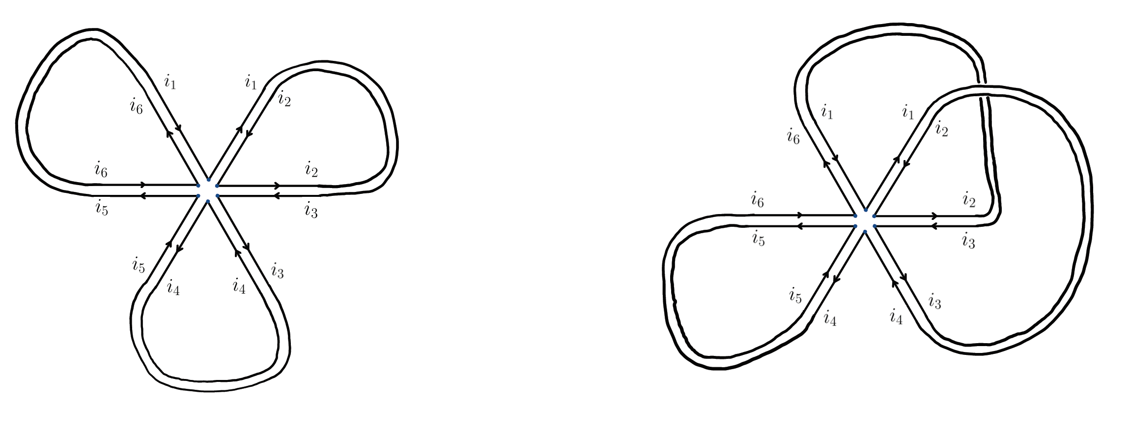
The leftmost diagram corresponds to the term $\langle X_{i_1 i_2}X_{i_2 i_3}\rangle_n \langle X_{i_3 i_4}X_{i_4 i_5}\rangle_n \langle X_{i_5 i_6}X_{i_6 i_1} \rangle_n$; we see that this term is only nonvanishing when $i_1=i_3=i_5$, and for any $i_2,i_4,i_6$. Thus, the diagram contributes a factor of $n$ to $\langle \textit{tr} X^6 \rangle_n$. On the other hand, the diagram on the right corresponds to the pairing $\langle X_{i_1 i_2}X_{i_3 i_4}\rangle_n \langle X_{i_2 i_3}X_{i_6 i_1}\rangle_n \langle X_{i_4 i_5}X_{i_6 i_6}\rangle_n$, which is only nonvanishing when $i_1 = i_4 = i_6 = i_3 = i_2$, and for any $i_5$. It follows that this diagram contributes a factor of $1/n$, which will vanish in the large $n$ limit, as the diagram is non-planar.
Finally, we can conclude that
Theorem 1.3. \begin{equation} \langle\text{tr} X^{2k}\rangle_n = \sum_{g=0}^{[k/2]} \varepsilon_g(k) n^{1-2g}, \end{equation} where $\varepsilon_g(k)$ is the number of labelled one-face maps with $k$ edges of genus $g$.
In particular, \begin{equation} \frac{1}{n}\langle \text{tr} X^{2k}\rangle_n = \varepsilon_0(k) + o(1/n), \end{equation} where $\varepsilon_0(k)$ is the number of planar labelled one-face maps with $k$ edges. For this reason, the large $n$ limit is sometimes referred to as the planar limit. It is well-known that $\varepsilon_0(k) = C_k$, the $k^{th}$ Catalan number.
$2.$ Matrix Ensembles and Orthogonal Polynomials.
Most computations within the scheme matrix ensembles are performed with techniques from the theory of orthogonal polynomials. Let us illustrate this connection in several different ways. Let us consider the Hermitian ensemble with measure \begin{equation*} \label{V-ensemble} d\mathbb{P}n(X) = \frac{1}{Z_n} e^{-\text{tr} Q(X)} dX, \end{equation*} where $Q(X) = X^{2n} + \cdots$ is a monic polynomial of even degree. Along with this ensemble, we also consider the family of monic orthogonal polynomials ${\pi_n(\lambda)}$, which satisfy the relation \begin{equation}\label{Q-OP} (\pi_m,\pi_n) := \int{\mathbb{R}}d\lambda e^{-Q(\lambda)} \pi_n(\lambda)\pi_m(\lambda) = h_n \delta_{nm}, \end{equation} where $V(\lambda)$ is the same polynomial, but in the real variable $\lambda$ instead of the matrix variable $X$. Our first connection between the ensemble defined by the above measure and the polynomials ${\pi_n(\lambda)}$ is given by the following theorem:
Theorem 2.1. (Heine’s formula) The polynomials $\pi_n(x)$ satisfy \begin{equation} \pi_n(\lambda) = \langle \det(\lambda - X)\rangle_n. \end{equation}
Proof. The proof is rather straightforward; first, it is clear from its definition that the right hand side of the above equation is a monic polynomial of degree $n$. Thus, we have only to show that this polynomial is orthogonal to $\lambda^m$, for $0 \leq m \leq n$. Suppose this is the case; then, \begin{align*} Z_n \cdot \big(\lambda^m, \langle \det(\lambda - X)n\big) &= \int{\mathbb{R}} d\lambda e^{-Q(\lambda)} \lambda^m\bigg[ \int_{\mathbb{R}^n}\prod_{i=1}^n d\lambda_i (\lambda - \lambda_i)e^{-Q(\lambda_i)} V^2(\lambda_1,\cdots,\lambda_n) \bigg] ; \end{align*} Note that $V(\lambda_1,\cdots,\lambda_n)\prod_{i=1}^n(\lambda - \lambda_i) = V(\lambda_1,\cdots,\lambda_n,\lambda)$, the Vandermonde determinant with one extra variable. Furthermore, the remaining piece of the integrand, $V(\lambda_1,\cdots,\lambda_n)\lambda^m$, can be rewritten as (labelling $\lambda = \lambda_{n+1}$): \begin{equation*} V(\lambda_1,\cdots,\lambda_n)\lambda^m = \frac{1}{n+1}\sum_{i=1}^{n+1} (-1)^{i+n+1} V(\lambda_1,\cdots, \hat{\lambda_i},\cdots,\lambda_{n+1})\lambda_i^m; \end{equation*} This is the expression for the determinant \begin{equation*} \begin{pmatrix} 1 & \lambda_1 & \cdots & \lambda_1^{n-1} &\lambda_1^m\\\ 1 & \lambda_2 & \cdots & \lambda_2^{n-1} &\lambda_2^m\\\ \vdots & \vdots & \cdots & \ddots &\vdots\\\ 1 & \lambda_{n+1} & \cdots & \lambda_{n+1}^{n-1} &\lambda_{n+1}^m\\\ \end{pmatrix}; \end{equation*} Clearly, this expression vanishes if $m < n$, and so $\det(\lambda - X)_n$ is orthogonal to the first $m$ monomials, and is thus the (unique) monic orthogonal polynomial, $\pi_n(\lambda)$.
In the above proof, if $m=n$, by what we just argued, we have that \begin{align*} Z_n \cdot \big(\lambda^n, \langle \det(\lambda - X)n\big) &= \frac{1}{n+1}\int{\mathbb{R}}d\lambda e^{-Q(\lambda)} \bigg[ \int_{\mathbb{R}^n}\prod_{i=1}^n d\lambda_i e^{-Q(\lambda_i)} V^2(\lambda_1,\cdots,\lambda_n,\lambda) \bigg] \\\ &= \frac{1}{n+1} Z_{n+1}; \end{align*} furthermore, since $\big(\lambda^n, \langle \det(\lambda - X)\rangle_n\big) = \big(\lambda^n, \pi_n\big) = (\pi_n, \pi_n) = h_n$, we obtain that \begin{equation*} Z_{n+1} = (n+1)h_n; \end{equation*} We therefore obtain inductively a second important link between orthogonal polynomials and matrix models:
Theorem 2.2. The partition function of the matrix model defined above is related to the orthogonality constants ${h_k}$ by \begin{equation} Z_n = n! \prod_{k=0}^n h_k. \end{equation}
We wish to make one final connection between matrix models and orthogonal polynomials. Consider the probability density function on the eigenvalues for this ensemble: \begin{equation} \rho_n(\lambda_1,\cdots, \lambda_n) := \frac{1}{Z_n} V^2(\lambda_1 ,\cdots,\lambda_n) e^{-\sum_{k=1}^n Q(\lambda_k)}. \end{equation} Recall that the Vandermonde determinant is the determinant of the matrix $\big(\lambda_i^{j-1} \big)$. Note that we can add any scalar multiple of any row/column to any other row/column without changing the determinant; thus, \begin{equation*} \det \begin{pmatrix} 1 & \lambda_1 & \cdots & \lambda_1^{n-1}\\\ 1 & \lambda_2 & \cdots & \lambda_2^{n-1}\\\ \vdots & \vdots & \ddots &\vdots\\\ 1 & \lambda_{n} & \cdots & \lambda_{n}^{n-1}\\\ \end{pmatrix} = \det \begin{pmatrix} p_0(\lambda_1) & p_1(\lambda_1) & \cdots & p_{n-1}(\lambda_1)\\\ p_0(\lambda_2) & p_1(\lambda_2) & \cdots & p_{n-1}(\lambda_2)\\\ \vdots & \vdots & \ddots &\vdots\\\ p_0(\lambda_n) & p_1(\lambda_n) & \cdots & p_{n-1}(\lambda_n)\\\ \end{pmatrix}, \end{equation*} for any family of monic polynomials ${p_{k}(\lambda)}$. In particular, we will choose $p_{k}(\lambda) = \pi_k(\lambda)$, the monic orthogonal polynomials with respect to the weight $e^{Q(\lambda)}$. Combining these two determinants, the density function becomes \begin{align*} \rho_n(\lambda_1,\cdots, \lambda_n) &= \frac{1}{Z_n} \det(\pi_k(\lambda_i))\det(\pi_k(\lambda_j)) e^{-\sum_{k=1}^n Q(\lambda_k)}\\\ &=\frac{1}{n! \prod_{k=0}^n h_k} \det\bigg(\sum_{k=0}^{n-1} \pi_k(\lambda_i)\pi_k(\lambda_j)\bigg) e^{-\sum_{k=0}^{n-1} Q(\lambda_k)}\\\ &=\frac{1}{n!} \det\bigg(\sum_{k=0}^{n-1} \frac{\pi_k(\lambda_i)\pi_k(\lambda_j)}{h_k}\bigg)e^{-\sum_{k=0}^{n-1} Q(\lambda_k)}\\\ &=\frac{1}{n!} \det\bigg(\sum_{k=0}^{n-1} \frac{\pi_k(\lambda_i)e^{-Q(\lambda_i)/2}\pi_k(\lambda_j)e^{-Q(\lambda_j)/2}}{h_k}\bigg)\\\ &:=\frac{1}{n!}\det(K(\lambda_i,\lambda_j)). \end{align*} The function \begin{equation} K(\lambda,\mu) := \sum_{k=0}^{n-1} \frac{\pi_k(\lambda)\pi_k(\mu)}{h_k}e^{-Q(\lambda)/2}e^{-Q(\mu)/2} \end{equation} is called the Christoffel-Darboux kernel; it acts as a projector onto the span of the first $n$ orthogonal polynomials, multiplied by $e^{Q/2}$. If $m < n$, integrating out the last $(n-m)$ variables, one finds that the joint density of the first $m$ eigenvalues is \begin{equation} \rho_n(\lambda_1,\cdots,\lambda_m) = \frac{(n-m)!}{n!} \det(K(\lambda_i,\lambda_j))_{i,j = 1}^m. \end{equation}
$3.$ Coulomb Gas Formalism.
In random matrix theory, one is often interested in the large n (planar) limit of certain quantities; by the previous section, we are equivalently looking for asymptotic formulae for orthogonal polynomials. One technique for addressing such questions is the coulomb gas method. For sake of clarity, we will focus our attention on one particular object, and its asymptotics: the free energy: \begin{align*} F = \frac{1}{n^2}\log Z_n = \frac{1}{n^2} \log \int_{\mathbb{R}^n} V(\lambda_1,\cdots,\lambda_n) e^{-n\sum_{i=1}^nQ(\lambda_i)} d\lambda_1\cdots d\lambda_n. \end{align*} Moving the Vandermonde determinant into the exponent, we can rewrite the free energy as \begin{align*} \frac{1}{n^2} \log \int_{\mathbb{R}^n} e^{-n^2 E(\lambda_1,\cdots,\lambda_n)}d\lambda_1\cdots d\lambda_n, \end{align*} where \begin{equation} E(\lambda_1,\cdots,\lambda_n) := \frac{1}{n^2}\sum_{i\neq j} \log \frac{1}{\lambda_i - \lambda_j} + \frac{1}{n}\sum_{i=1}^n Q(\lambda_i). \end{equation} The above sum can be interpreted as an energy functional for a system of $n$ charges interacting via the $2D$ Coulomb potential. The fact that the $\lambda_i’s$ are real translates to the condition that the charges are confined to live on a wire (the real line). The charges all have mass $1/n$, and all have the same sign, and so the affect of the coulomb interaction is repulsive. On the other hand, the charges sit in a background confining potential $Q(\lambda)$, which holds them together. Note that both terms in $E(\lambda_1,\cdots,\lambda_n)$ are of order 1, by how we scaled $Q\to nQ$.
With this interpetation in mind, let us turn our attention back to the free energy. When $n$ is very large, typical saddle point analysis tells us that we expect the dominant contributions to the free energy to come from the minima of $E$, i.e. \begin{align*} F &= \frac{1}{n^2} \log \int_{\mathbb{R}^n} e^{-n^2E(\lambda_1,\cdots\lambda_n)} d\lambda_1\cdots d\lambda_n\\\ &\sim \frac{1}{n^2} \log e^{-n^2 \min E(\lambda_1,\cdots\lambda_n)}\\\ &= \min E(\lambda_1,\cdots\lambda_n). \end{align*} Writing the density of charges as a measure $\mu = \frac{1}{n}\sum_{k=1}^n \delta_{{\lambda_{k}}}$, we can rewrite this minimization problem as \begin{align*} \min E(\lambda_1,\cdots\lambda_n) &= \min \frac{1}{n^2}\sum_{i\neq j} \log \frac{1}{\lambda_i - \lambda_j} + \frac{1}{n}\sum_{i=1}^n Q(\lambda_i)\\\ &= \min_{\mu(\mathbb{R}) = 1} \int\int \log\frac{1}{x-y} d\mu(x) d\mu(y) + \int Q(x) d\mu(x). \end{align*} As $n \to \infty$, we expect that the charges should coalesce into a continuous distribution of charge $\mu$, i.e., $ \frac{1}{n}\sum_{k=1}^n \delta_{{\lambda_{k}}} \to \rho(x) dx$, where $\rho$ has total charge $1$. This sort of equilibrium problem is well-known in potential theory; we can use our physical intuition to try and find its solution. In equilibrium, the effective potential (the potential coming from the charges themselves, plus the external field) should be constant on the support of the charges, otherwise the charges would move around, and we wouldn’t be in equilibrium. This yields the following equilibrium condition: \begin{equation} U^\mu(x) + Q(x) = \text{const.}, \end{equation} for $x$ in the support of the charges. Here, $U^\mu(x)$ is the potential given off by the charges: \begin{equation} U^\mu(x) = \int \log\frac{1}{x-y} d\mu(y). \end{equation} Differentiating the equilibrium condition, we obtain the equation \begin{equation} C^\mu(x) + Q’(x) = 0, \end{equation} where $C^\mu(x)$ is the Cauchy transform of the measure $\mu$: \begin{equation} C^\mu(x) = \int \frac{d\mu(y)}{y-x}, \end{equation} considered here in the principal value sense. We are almost at our goal; all that remains is to recover the measure $\mu$ from the above formula, and then plug it back in to the energy functional, and then we have our expression for the dominant contribution to the free energy. But how do we recover a measure if we know its Cauchy transform? Luckily, this question has already been answered for us; these are the famous Sokhotsky-Plemelj formulae: \begin{align*} \frac{d\mu(x)}{dx} &= \frac{1}{2\pi i}\bigg( C^\mu_+(x) - C^\mu_-(x)\bigg),\\\ P.V.\int \frac{d\mu(y)}{y-x} &= C^\mu_+(x) + C^\mu_-(x), \end{align*} for $x$ in the support of the charges. These formulae, along with a little knowledge of complex analysis, will allow us to recover $d\mu(x) = \rho(x)dx$. Consider the function $P(z):=Q’(z)C^{\mu}(z) - (C^\mu(z))^2$. This function is analytic everywhere in the complex plane, except possibly at the places where $C^\mu(z)$ loses analyticity–the support of the charges. Let us compute the jump of $P(z)$ across the support: \begin{align*} P_+(z) - P_-(z) &= Q’(z)\bigg(C^{\mu}+(z)-C^{\mu}-(z)\bigg) - (C^\mu_+(z))^2 + (C^\mu_-(z))^2\\\ &= \bigg(C^{\mu}+(z)+C^{\mu}-(z)\bigg)\bigg(C^{\mu}+(z)-C^{\mu}-(z)\bigg)- (C^\mu_+(z))^2 + (C^\mu_-(z))^2\\\ &=0, \end{align*} and so $P(z)$ is continuous across the support of the charges, and thus continuous everywhere. By Morera’s theorem, $P(z)$ is an entire function. Furthermore, we know the exact growth rate of $P(z)$ at infinity: $P(z) = \mathcal{O}(z^{n-2})$, where $\deg Q = n$. Thus, by Liouville’s theorem, $P(z)$ is a polynomial of degree $n-2$. We thus have obtained an algebraic equation for $C^\mu(z)$: \begin{equation} (C^\mu(z))^2 - Q’(z)C^{\mu}(z) - P(z) = 0; \end{equation} this equation is quadratic in $C^\mu(z)$, and thus can be solved: \begin{equation} C^{\mu}(z) = -\frac{1}{2}Q’(z) \pm \frac{1}{2}\sqrt{Q’(z)^2 - 4P(z) \end{equation} Therefore, by the other half of the Sokhotsky-Plemelj formulae, we can recover the density: \begin{equation} \rho(x) = \frac{d\mu(x)}{dx} = \frac{1}{2\pi} \sqrt{4P(x) - Q’(x)^2}. \end{equation} In practice, computing the coefficients of $P(x)$ is not a trivial task, especially if the support of the measure is more than one interval. However, if the potential $Q(x)$ is partiularly simple, the computations can be done rather quickly; if $Q(x) = \frac{1}{2}x^2$, as it is for the GUE, then it is easy to see that $P(x) = 1$, and so the formula above becomes \begin{equation} \rho(x) = \frac{1}{2\pi}\sqrt{4-x^2}; \end{equation} this is Wigner’s semicircle law.
$4.$ 2-Matrix Models.
We now discuss $N$-matrix models, which are matrix models $n$ over copies of $\mathcal{H}$n; for simplicity, we specialize to the case of $N = 2$. We denote the matrices in the first copy of $\mathcal{H}$n by $A$, and in the second copy by $B$. The probability measure we consider here is \begin{equation*} d\mathbb{P}n(A,B) = \frac{1}{Z_n} \exp\bigg( -\frac{n}{2} \text{tr} (A^2 + B^2 + 2cAB)\bigg) dA dB. \end{equation*} The quantity in the exponent can be thought of as a quadratic form on pairs of Hermitian matrices $(A,B)$, with defining matrix \begin{equation*} \label{quad-form} \begin{pmatrix} 1 & c \\\ c & 1 \end{pmatrix}. \end{equation*} Expected values are denoted in the same way as before; this ensemble is also Gaussian in nature, and so the matrix version of Wick’s theorem applies. As before, all one-point functions vanish identically. Thus, the relevant expected values to compute are the two-point functions; they are: \begin{align*} \langle A{i_1j_1}A_{i_2j_2}\rangle_n = \langle B_{i_1j_1}B_{i_2j_2}\rangle_n &= \frac{1}{n}\frac{1}{1-c^2} \delta_{i_1 j_2}\delta_{i_2 j_1},\\\ \langle A_{i_1j_1}B_{i_2j_2}\rangle_n &= \frac{1}{n}\frac{c}{1-c^2} \delta_{i_1 j_2}\delta_{i_2 j_1}. \end{align*} The computations are almost identical to the $1$-matrix case, and so we omit them here (the process involves the extra step of diagonalizing the quadratic form above. The crucial point here is that the two point functions for “like” matrices are the same, and differ from the two point function for the “mismatched” matrices by an overall constant. Therefore, the same sorts of combinatorial identites that held before for the correlations now hold for graphs with two possible weights on the vertices.
This connection of the 2-matrix model to enumeration of 2-colored graphs was exploited by V. Kazakov to answer questions about the Ising model on random planar graphs.
$5.$ Itzykson-Zuber Integral over the Unitary Group.
With this combinatorial interpretation of the model in mind, we would like to go about explicitly computing certain matrix integrals. To do this, we will need to switch over to eigenvalue variables; this is not as trivial as a task as it was in the 1-matrix case. This is made apparent as follows. Suppose we want to compute the expected value of some function $f(A,B) = f(\text{tr} A,\text{tr} B)$. This is written as \begin{equation} \langle f(A,B) \rangle_n = \frac{1}{Z_n}\int_{A\in \mathcal{H}n} \int{B \in \mathcal{H}n}dA dB \exp\bigg( -\frac{n}{2} \text{tr} (A^2 + B^2 + 2cAB)\bigg) f(A,B). \end{equation} Letting $A = U^\dagger X U$, $B = V^\dagger Y V$, where $X = \text{diag}(x_1,\cdots,x_n)$, $Y = \text{diag}(y_1,\cdots,y_n)$ are diagonal matrices, we see that the above is \begin{align*} =& \frac{1}{Z_n}\int{X,Y\in \mathbb{R}^n} dX dY V(X)^2V(Y)^2f(X,Y) \exp\bigg( -\frac{n}{2} \text{tr} (X^2 + Y^2)\bigg) \\\ &\times\int_{U,V \in U(n)/U_{diag}(n)} dU dV \exp\big(nc \text{tr} AB\big) \end{align*} We must pay careful attention to the integral \begin{equation*} \int_{U,V \in U(n)/U_{diag}(n)} dU dV \exp\big(nc \text{tr} AB\big) = \int_{U,V \in U(n)/U_{diag}(n)} dU dV \exp\big(nc \text{tr} U^\dagger X UV^\dagger Y V\big). \end{equation*} Making the change of variables in $V$: $W = UV^\dagger$, and integrating over $U$ first (and applying translation invariance of the Haar measure), we see that the above integral becomes \begin{equation} \text{vol}(U(n)/U_{diag}(n)) \cdot \int_{W \in U(n)/U_{diag}(n)} dW \exp\big(nc \text{tr} X W Y W^\dagger\big), \end{equation} where $X,Y$ are diagonal matrices, and $W$ is unitary. Integrals of this type are called Harish-Chandra or Itzykson-Zuber integrals over the unitary group. It turns out that such integrals can be computed explicitly. We will consider here a slight generalization of the above: \begin{equation} I(A,B;s) := \int_{U(n)/U_{diag}(n)} dU \exp\big(s \text{tr} A U B U^\dagger\big), \end{equation} where $A, B$ are Hermitian matrices. Our claim is the following:
Theorem 5.1. Let $I(A,B;s)$ be as defined above, and suppose $A$ has eigenvalues $a_1,\cdots, a_n$, and $B$ has eigenvalues $b_1,\cdots, b_n$. Then \begin{equation} I(A,B;s) = s^{-n(n-1)/2} \frac{\det(e^{a_ib_j})}{V(a) V(b)}. \end{equation}
The remainder of this section is dedicated to a proof of this fact. We use the heat kernel technique, which is outlined in a wonderful paper by P. Zinn-Justin and J.B. Zuber. Consider the heat equation in the variable $A$: \begin{equation}\label{heat-eq-1} \begin{cases} \left( \frac{\partial}{\partial t} - \frac{1}{2} \Delta_A \right) u(A,t) = 0,\\\ u(A,0) = f(A). \end{cases} \end{equation} Here, $\Delta_A$ is the usual Laplace operator on $\mathcal{H}n$: \begin{equation*} \Delta{A} = \sum_{i=1}^n \frac{\partial^2}{\partial A_{ii}^2} + \frac{1}{2}\sum_{i < j}\left(\frac{\partial^2}{\partial \text{Re}(A_{ij})^2} + \frac{\partial^2}{\partial \text{Im}(A_{ij})^2}\right). \end{equation*} The heat kernel for this operator is easily derived (since $\mathcal{H}n \cong \mathbb{R}^{n^2}$ in scaled coordinates): \begin{equation*} K(A,B;t) = \frac{1}{(2\pi t)^{n^2/2}}\exp\left(\frac{1}{2t} \text{tr}(A-B)^2\right); \end{equation*} The solution to the heat equation above is thus given by \begin{equation*} u(A,t) = \int{\mathcal{H}n} dB f(B) \frac{1}{(2\pi t)^{n^2/2}}\exp\left(-\frac{1}{2t} \text{tr}(A-B)^2\right). \end{equation*} Let us suppose the initial data $f(A)$ depends only on the eigenvalue variables, i.e. $f(A) = f(\text{tr}(A))$. Then, converting the above to eigenvalue variables $A = U^\dagger X U$, $B = V^\dagger Y V$, we find that \begin{align*}\label{heat2} u(A,t) = &\frac{1}{(2\pi t)^{n^2/2}}\int{\mathbb{R}^n} dY, V^2(Y)f(Y) \exp\left(-\frac{1}{2t} \text{tr}(X^2 + Y^2) \right) \\\ &\times\int_{U(n)/U_{diag}(n)} dW \exp\big(\frac{1}{t} \text{tr} X W Y W^\dagger\big), \end{align*} where $W = UV^\dagger$. Note that the inner integral is the object we want to compute. Furthermore, the above formula implies that if $f(U^\dagger X U) = f(X)$, then $u(U^\dagger X U,t) = u(X,t)$ for all $t > 0$ as well. Let us see examine the above equation in eigenvalue coordinates. With the help of the formula we derived for the laplacian on the eigenvalue coordinates, we find that \begin{align*} 0 &= \left( \frac{\partial}{\partial t} - \frac{1}{2} \Delta_A \right) u(A,t) = \left( \frac{\partial}{\partial t} - \frac{1}{2} \Delta_{X} \right) u(X,t)\\\ &= \frac{\partial u }{\partial t} - \frac{1}{2}\frac{1}{V^2(X)}\sum_{i=1}^n\frac{\partial}{\partial x_i} \left(V^2(X) \frac{\partial u}{\partial x_i} \right)\\\ &= \frac{\partial u }{\partial t} - \frac{1}{2}\frac{1}{V^2(X)}\sum_{i=1}^n \left(2V(X)\frac{\partial V}{\partial x_i} \frac{\partial u}{\partial x_i} + V^2(X) \frac{\partial^2 u}{\partial x_i^2}\right); \end{align*} Multiplying the above equation by the Vandermonde determinant $V(x)$, and using the fact that $\sum_{i=1}^n \frac{\partial^2 V}{\partial x_i^2}= 0$, the above equation becomes \begin{align*} 0 &= \frac{\partial V u }{\partial t} - \frac{1}{2}\sum_{i=1}^n \left(2\frac{\partial V}{\partial x_i} \frac{\partial u}{\partial x_i} + V(X)\frac{\partial^2 u}{\partial x_i^2}\right)\\\ &= \frac{\partial V u }{\partial t} - \frac{1}{2}\sum_{i=1}^n \left(\underbrace{u\frac{\partial^2 V}{\partial x_i^2}}{=0} + 2\frac{\partial V}{\partial x_i} \frac{\partial u}{\partial x_i} + V(X)\frac{\partial^2 u}{\partial x_i^2}\right)\\\ &= \left(\frac{\partial}{\partial t} - \frac{1}{2} \sum{i=1}^n \frac{\partial^2}{\partial x_i^2}\right)V(X)u(X,t), \end{align*} and so $V(x)u(X,t)$ satisfies a heat equation of a different form. The generic solution for initial data $g(X)$ to the above heat equation is \begin{equation*} h(X,t) = \int_{Y\in \mathbb{R}^n} dY \frac{1}{(2\pi t)^{n/2}}\exp\left(-\frac{1}{2t}\text{tr}(X-Y)^2\right) g(Y); \end{equation*} In particular, for initial data $g(X) = V(X)f(X)$, we obtain the formula \begin{equation}\label{heat3} V(X)u(X,t) = \int_{Y\in \mathbb{R}^n} dY \frac{1}{(2\pi t)^{n/2}}\exp\left(-\frac{1}{2t}\text{tr}(X-Y)^2\right) V(Y)f(Y) \end{equation} multiplying the previous equation by $V(X)$, we see that we have two expressions for the same function, $V(X)u(X,t)$. Equating these expressions yields \begin{align*} &V(X)\frac{1}{(2\pi t)^{n^2/2}}\int_{\mathbb{R}^n} dY V^2(Y)f(Y) \exp\left(-\frac{1}{2t} \text{tr}(X^2 + Y^2) \right) \int_{U(n)/U_{diag}(n)} dW \exp\big(\frac{1}{t} \text{tr} X W Y W^\dagger\big)\\\ &= u(X,t)=\int_{Y\in \mathbb{R}^n} dY \frac{1}{(2\pi t)^{n/2}}\exp\left(-\frac{1}{2t}\text{tr}(X-Y)^2\right) V(Y)f(Y). \end{align*} Setting $f(Y) = \delta(Y-Y_0)$, we obtain that \begin{align*} &V(X)V^2(Y_0)\frac{1}{(2\pi t)^{n^2/2}}\exp\left(-\frac{1}{2t} \text{tr}(X^2 + Y_0^2) \right) \int_{U(n)/U_{diag}(n)} dW \exp\big(\frac{1}{t} \text{tr} X W Y_0 W^\dagger\big)\\\ &= \frac{1}{(2\pi t)^{n/2}}\exp\left(-\frac{1}{2t}\text{tr}(X-Y_0)^2\right) V(Y_0). \end{align*} Rearranging, and relabelling $Y_0 = Y$, we get \begin{equation*} \int_{U(n)/U_{diag}(n)} dW \exp\big(\frac{1}{t} \text{tr} X W Y W^\dagger\big) = (2\pi t)^{-n(n-1)/2}\frac{\exp(\frac{1}{t}\text{tr} XY)}{V(Y) V(X)}; \end{equation*} finally, \begin{equation} \int_{U(n)/U_{diag}(n)} dW \exp\big(\frac{1}{t} \text{tr} X W Y W^\dagger\big) = (2\pi t)^{-n(n-1)/2}\frac{\det e^{\frac{1}{t}x_iy_j }}{V(Y) V(X)}. \end{equation}
$6.$ 2-Matrix Models and Biorthogonal Polynomials.
Just as $1$-matrix models are connected to orthogonal polynomials, $2$-matrix models are connected to biorthogonal polynomials. Consider again the $2$-matrix model defined by the measure \begin{equation*} d\mathbb{P}n(A,B) = \frac{1}{Z_n} \exp\bigg( -\frac{n}{2} \text{tr} (A^2 + B^2 + 2cAB)\bigg) dA dB, \end{equation*} and recall that expected values of invariant functions $f(A,B) = f(\text{tr}(A),\text{tr}(B))$ are given by the formula \begin{equation*} \langle f(A,B) \rangle_n = \frac{1}{Z_n}\int{A\in \mathcal{H}n} \int{B \in \mathcal{H}n}dA dB \exp\bigg( -\frac{n}{2} \text{tr} (A^2 + B^2 + 2cAB)\bigg) f(A,B). \end{equation*} Letting $A = U^\dagger X U$, $B = V^\dagger Y V$, where $X = \text{diag}(x_1,\cdots,x_n)$, $Y = \text{diag}(y_1,\cdots,y_n)$ are diagonal matrices, we can integrate out eigenvalue variables to obtain \begin{align*} &= \frac{1}{Z_n’}\int{X,Y\in \mathbb{R}^n} dX dY V(X)^2V(Y)^2f(X,Y) \exp\bigg( -\frac{n}{2} \text{tr} (X^2 + Y^2)\bigg) \\\ &\times\int_{U \in U(n)/U_{diag}(n)} dW \exp\big(nc \text{tr} XWYW^\dagger\big). \end{align*} The integral inside is precisely the Itzykson Zuber integral we computed previously; we insert the expression we derived for it into the above formula, absorbing all constant factors into the partition function: \begin{align*} \langle f(A,B) \rangle_n &= \frac{1}{Z_n’’}\int_{X,Y\in \mathbb{R}^n} dX dY V(X)^2V(Y)^2f(X,Y) \exp\bigg( -\frac{n}{2} \text{tr} (X^2 + Y^2)\bigg) \frac{\det e^{nc x_iy_j }}{V(Y) V(X)}\\\ &=\frac{1}{Z_n’’}\int_{X,Y\in \mathbb{R}^n} \prod_{k=1}^n dx_k dy_k f(x,y) V(x)V(y)\exp\bigg( -\frac{n}{2} \sum_{k=1} x_i^2 + y_i^2 + 2ncx_i y_i\bigg). \end{align*}
Thus, just as we were able to connect the 1-matrix model and orthogonal polynomials, we can connect the 2-matrix to bi-orthogonal polynomials; i.e., the polynomials $p_n(x),q_n(y)$ satisfying \begin{align*} \int_{\mathbb{R}} \int_{\mathbb{R}} p_n(x)q_n(y) e^{-\frac{n}{2}x^2-\frac{n}{2}y^2-2nxy} dxdy = h_n \delta_{nm} \end{align*} Of course, the same sorts of arguments can be made for more general potentials besides $x^2,y^2$; we postpone discussion of this to a later entry.